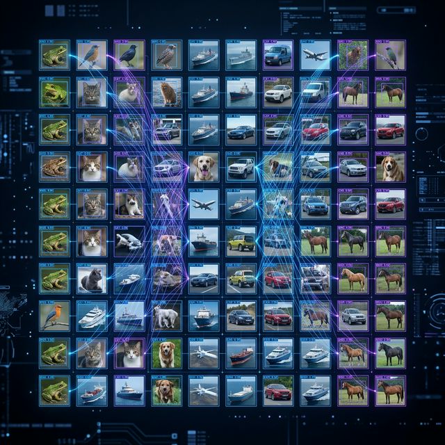
Computer Vision Experiments: CIFAR-10 Classification

1# Computer Vision Experiments: CIFAR-10 Classification
2
3This repository contains a comparative study between a traditional Computer Vision approach (HOG + SVM) and a Deep Learning approach (CNN) for image classification on the CIFAR-10 dataset.
4
5## Project Overview
6
7The objective is to evaluate and compare the performance of two distinct methodologies for object recognition:
81.  **Traditional CV**: Histogram of Oriented Gradients (HOG) features combined with a Support Vector Machine (SVM) classifier.
92.  **Deep Learning**: A Convolutional Neural Network (CNN) architecture implemented using TensorFlow/Keras.
10
11## Dataset
12
13- **Dataset**: CIFAR-10
14- **Size**: 60,000 32x32 color images in 10 classes.
15- **Split**: 50,000 training images and 10,000 test images.
16- **Preprocessing**: Normalization of pixel values to [0, 1] and one-hot encoding of labels for the CNN.
17
18## Methodology
19
20### 1. HOG + SVM (Traditional)
21- **Feature Extraction**: HOG features were extracted from grayscale versions of the images.
22- **Parameters**: `orientations=9`, `pixels_per_cell=(8, 8)`, `cells_per_block=(2, 2)`.
23- **Classifier**: SVM with a linear kernel and regularization parameter `C=1.0`.
24
25### 2. CNN (Deep Learning)
26- **Architecture**:
27    - 3 Convolutional Layers (32, 64, and 128 filters) with ReLU activation.
28    - MaxPooling layers after each convolution.
29    - Flattening and a Dense layer (128 units) with Dropout (0.5).
30    - Softmax output layer (10 units).
31- **Training**: Adam optimizer, categorical crossentropy loss, `BATCH_SIZE=64`, `EPOCHS=10`.
32
33## Key Results
34
35| Metric | HOG + SVM | CNN (Final Epoch) |
36| :--- | :--- | :--- |
37| **Accuracy** | 53.01% | 71.33% (Validation) |
38| **Precision** | 52.72% | - |
39| **Recall** | 53.01% | - |
40| **F1-Score** | 52.72% | - |
41
42- **Training Time**: SVM took ~600 seconds, while CNN took ~788 seconds for 10 epochs.
43- **Analysis**: The CNN significantly outperformed the HOG+SVM approach, achieving over 70% validation accuracy, demonstrating the superior feature extraction capabilities of deep learning for complex image datasets like CIFAR-10.
44
45## Files
46- `Computer_Vision_Experiments.ipynb`: The main notebook containing the implementation and evaluation.
47- `Object Recognition A Comparative Study of HOG Features and Deep Learning Approaches.pdf`: Summary report of the findings.
48
49## How to Run
501.  Open `Computer_Vision_Experiments.ipynb` in Jupyter or Google Colab.
512.  Ensure you have `tensorflow`, `scikit-learn`, `scikit-image`, and `matplotlib` installed.
523.  Run all cells to replicate the experiments and view results.
53